Coherence Factor for Ultrasound Beamforming

This example demonstrates different coherence factor formulations and their applications in ultrasound imaging. Coherence factors measure the degree to which signals from different array elements are in phase, providing quality metrics for adaptive beamforming and aberration correction.

We’ll explore:

• Different coherence scenarios (perfect to severely aberrated)

• Multiple coherence factor types (Standard, Generalized, Sign, Phase)

• Parameter effects and practical considerations

This example demonstrates coherence factor calculations for beamforming quality assessment [1], with applications to aberration correction [2]. We compare different formulations including the generalized coherence factor [3] and phase coherence methods [4].

References

[1]

Rigby, K. W., et al. (1999). Improved in vivo abdominal image quality using real-time estimation and correction of wavefront aberration. Proceedings IEEE Ultrasonics Symposium, 2, 1351-1355.

[2] (1,2)

Vr˚alstad, A.E. et al. (2024). Coherence Based Sound Speed Aberration Correction — with clinical validation in fetal ultrasound. arXiv:2411.16551

[3]

Li, P. C., & Li, M. L. (2003). Adaptive imaging using the generalized coherence factor. IEEE UFFC, 50(2), 128-141.

[4]

Camacho, J., et al. (2009). Phase coherence imaging. IEEE UFFC, 56(5), 958-974.

Example

# Note: it would probably be interesting to use a PICMUS dataset with a beamformer
# at some point.

1. Import required modules and functions

import matplotlib

matplotlib.use("Agg")  # Use non-interactive backend
import matplotlib.pyplot as plt
import numpy as np
from scipy import ndimage

from ultrasound_metrics.metrics.coherence import (
    coherence_factor,
    generalized_coherence_factor,
    phase_coherence_factor,
    sign_coherence_factor,
)

2. Setup: Simulate realistic ultrasound beamforming scenarios

# Define image dimensions and number of receive elements
height, width = 128, 96
n_elements = 32

# Create a base complex-valued signal pattern with point targets and speckle
np.random.seed(42)  # For reproducible results
base_signal = np.random.randn(height, width) + 1j * np.random.randn(height, width)
base_signal = base_signal.astype(np.complex64)

# Add some structured features (simulating point targets and speckle)
# Point target in upper region (high coherence expected)
base_signal[30:35, 45:50] += 5.0 + 5.0j

# Speckle pattern in middle region
y_speckle, x_speckle = np.mgrid[50:80, 20:75]
speckle_pattern = np.exp(1j * (x_speckle * 0.3 + y_speckle * 0.2))
base_signal[50:80, 20:75] += 2.0 * speckle_pattern

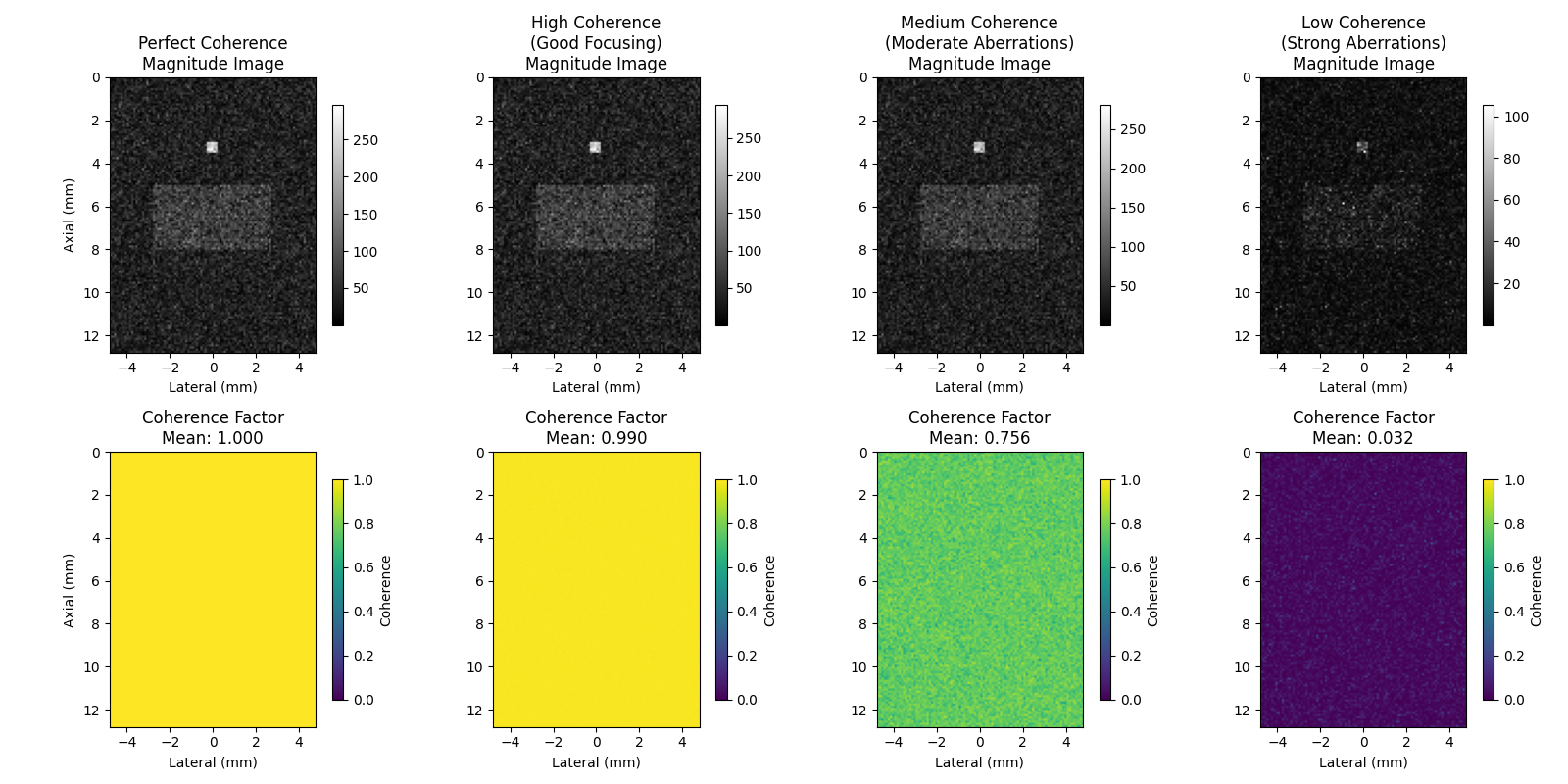
3. Create scenarios with different coherence levels

# These scenarios simulate different imaging conditions from ideal focusing
# to severe aberrations, showing how coherence factors respond to signal quality.

# Scenario 1: Perfect coherence (all elements receive identical signal)
beamsum_perfect = np.tile(base_signal[None, :, :], (n_elements, 1, 1))
coherence_perfect = coherence_factor(beamsum_perfect)

# Scenario 2: High coherence with small phase variations (good focusing)
beamsum_high = np.zeros((n_elements, height, width), dtype=np.complex64)
for i in range(n_elements):
    # Small random phase shifts (simulating good focusing)
    phase_noise = np.random.normal(0, 0.1, (height, width))  # Small phase variations
    beamsum_high[i] = base_signal * np.exp(1j * phase_noise)

coherence_high = coherence_factor(beamsum_high)

# Scenario 3: Medium coherence with moderate aberrations
beamsum_medium = np.zeros((n_elements, height, width), dtype=np.complex64)
for i in range(n_elements):
    # Moderate phase aberrations
    phase_aberration = np.random.normal(0, 0.5, (height, width))
    amplitude_variation = 1.0 + np.random.normal(0, 0.2, (height, width))
    beamsum_medium[i] = base_signal * amplitude_variation * np.exp(1j * phase_aberration)

coherence_medium = coherence_factor(beamsum_medium)

# Scenario 4: Low coherence (strong aberrations/noise)
beamsum_low = np.zeros((n_elements, height, width), dtype=np.complex64)
for i in range(n_elements):
    # Strong phase aberrations and amplitude variations
    phase_aberration = np.random.uniform(-np.pi, np.pi, (height, width))
    amplitude_variation = np.random.uniform(0.2, 1.8, (height, width))
    noise = 0.5 * (np.random.randn(height, width) + 1j * np.random.randn(height, width))
    beamsum_low[i] = base_signal * amplitude_variation * np.exp(1j * phase_aberration) + noise

coherence_low = coherence_factor(beamsum_low)

4. Visualize the coherence maps

fig, axes = plt.subplots(2, 4, figsize=(16, 8))

# Define extent for proper axis scaling (simulate realistic ultrasound coordinates)
lateral_extent = [-width / 2 * 0.1, width / 2 * 0.1]  # mm
axial_extent = [0, height * 0.1]  # mm
extent = [lateral_extent[0], lateral_extent[1], axial_extent[1], axial_extent[0]]

scenarios = [
    (beamsum_perfect, coherence_perfect, "Perfect Coherence"),
    (beamsum_high, coherence_high, "High Coherence\n(Good Focusing)"),
    (beamsum_medium, coherence_medium, "Medium Coherence\n(Moderate Aberrations)"),
    (beamsum_low, coherence_low, "Low Coherence\n(Strong Aberrations)"),
]

for idx, (beamsum, coherence, title) in enumerate(scenarios):
    # Top row: Magnitude of summed beamforming result
    summed_magnitude = np.abs(np.sum(beamsum, axis=0))

    im1 = axes[0, idx].imshow(summed_magnitude, cmap="gray", extent=extent)
    axes[0, idx].set_title(f"{title}\nMagnitude Image")
    axes[0, idx].set_xlabel("Lateral (mm)")
    if idx == 0:
        axes[0, idx].set_ylabel("Axial (mm)")
    plt.colorbar(im1, ax=axes[0, idx], shrink=0.8)

    # Bottom row: Coherence factor
    im2 = axes[1, idx].imshow(coherence, cmap="viridis", vmin=0, vmax=1, extent=extent)
    axes[1, idx].set_title(f"Coherence Factor\nMean: {coherence.mean():.3f}")
    axes[1, idx].set_xlabel("Lateral (mm)")
    if idx == 0:
        axes[1, idx].set_ylabel("Axial (mm)")
    plt.colorbar(im2, ax=axes[1, idx], shrink=0.8, label="Coherence")

plt.tight_layout()
plt.show()

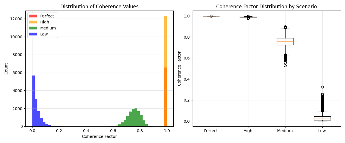
5. Analyze coherence distribution across scenarios

fig, axes = plt.subplots(1, 2, figsize=(12, 5))

# Histogram of coherence values
coherence_data = [
    (coherence_perfect.flatten(), "Perfect", "red"),
    (coherence_high.flatten(), "High", "orange"),
    (coherence_medium.flatten(), "Medium", "green"),
    (coherence_low.flatten(), "Low", "blue"),
]

for coherence_vals, label, color in coherence_data:
    # Use consistent binning across all datasets for fair comparison
    axes[0].hist(coherence_vals, bins=50, alpha=0.7, label=label, color=color, range=(0, 1), density=False)

axes[0].set_xlabel("Coherence Factor")
axes[0].set_ylabel("Count")
axes[0].set_title("Distribution of Coherence Values")
axes[0].legend()
axes[0].grid(True, alpha=0.3)

# Box plot comparison
coherence_values = [
    coherence_perfect.flatten(),
    coherence_high.flatten(),
    coherence_medium.flatten(),
    coherence_low.flatten(),
]
labels = ["Perfect", "High", "Medium", "Low"]

axes[1].boxplot(coherence_values, tick_labels=labels)
axes[1].set_ylabel("Coherence Factor")
axes[1].set_title("Coherence Factor Distribution by Scenario")
axes[1].grid(True, alpha=0.3)

plt.tight_layout()
plt.show()

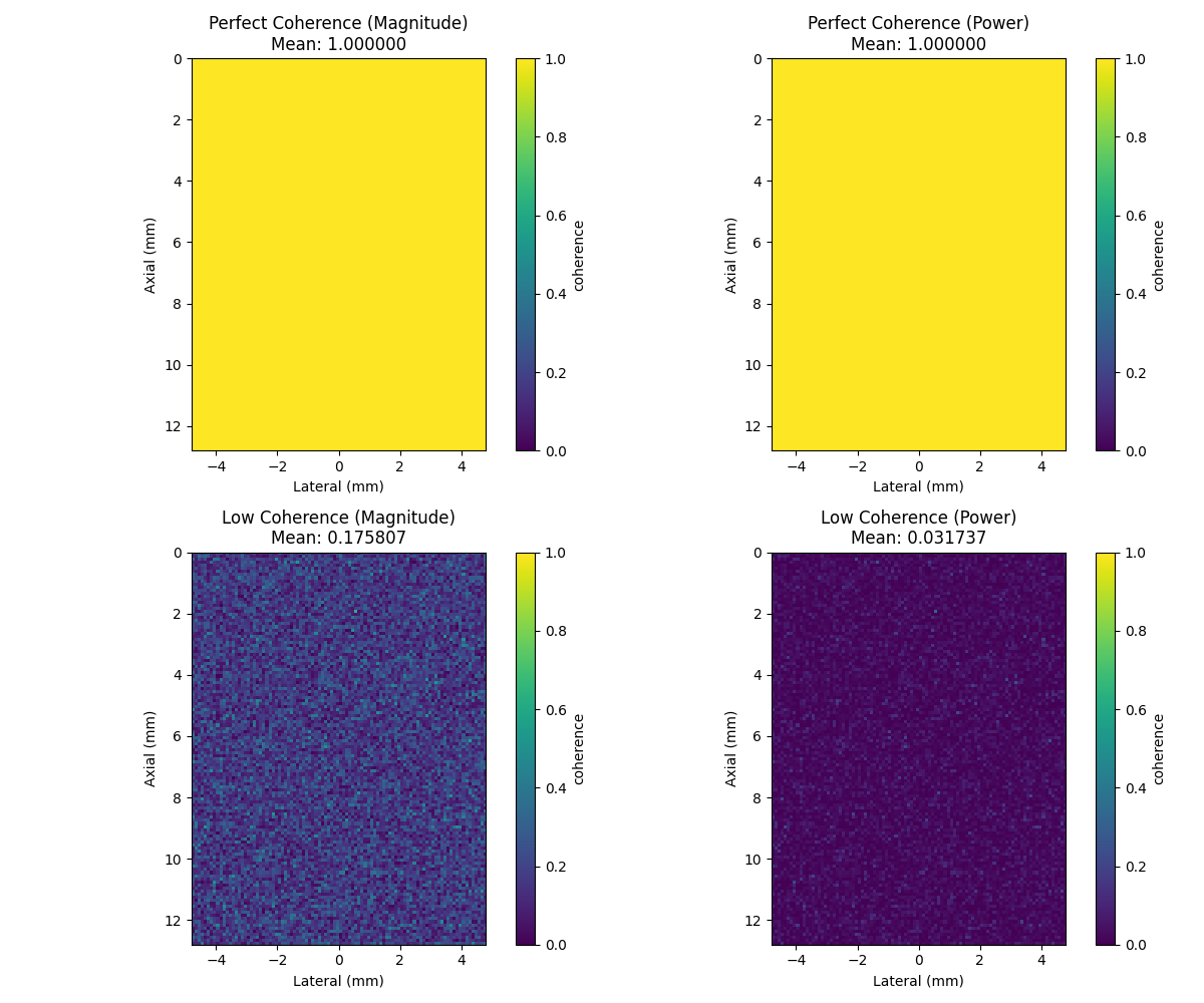
6. Compare magnitude-based vs power-based coherence formulations

Two mathematical formulations exist in the literature:

• Magnitude-based: CF = \|Σ s_i\| / Σ \|s_i\| (original formulation)

• Power-based: CF = \|Σ s_i\|² / (M * Σ \|s_i\|²) (vbeam library)

# Test with perfect coherence scenario
coherence_perfect_mag = coherence_factor(beamsum_perfect, power_based=False)
coherence_perfect_pow = coherence_factor(beamsum_perfect, power_based=True)

# Test with low coherence scenario
coherence_low_mag = coherence_factor(beamsum_low, power_based=False)
coherence_low_pow = coherence_factor(beamsum_low, power_based=True)

# Create comparison visualization
fig, axes = plt.subplots(2, 2, figsize=(12, 10))

# Perfect coherence comparison
im00 = axes[0, 0].imshow(coherence_perfect_mag, cmap="viridis", vmin=0, vmax=1, extent=extent)
axes[0, 0].set_title(f"Perfect Coherence (Magnitude)\nMean: {coherence_perfect_mag.mean():.6f}")
axes[0, 0].set_xlabel("Lateral (mm)")
axes[0, 0].set_ylabel("Axial (mm)")
plt.colorbar(im00, ax=axes[0, 0], label="coherence")

im01 = axes[0, 1].imshow(coherence_perfect_pow, cmap="viridis", vmin=0, vmax=1, extent=extent)
axes[0, 1].set_title(f"Perfect Coherence (Power)\nMean: {coherence_perfect_pow.mean():.6f}")
axes[0, 1].set_xlabel("Lateral (mm)")
axes[0, 1].set_ylabel("Axial (mm)")
plt.colorbar(im01, ax=axes[0, 1], label="coherence")

# Low coherence comparison
im10 = axes[1, 0].imshow(coherence_low_mag, cmap="viridis", vmin=0, vmax=1, extent=extent)
axes[1, 0].set_title(f"Low Coherence (Magnitude)\nMean: {coherence_low_mag.mean():.6f}")
axes[1, 0].set_xlabel("Lateral (mm)")
axes[1, 0].set_ylabel("Axial (mm)")
plt.colorbar(im10, ax=axes[1, 0], label="coherence")

im11 = axes[1, 1].imshow(coherence_low_pow, cmap="viridis", vmin=0, vmax=1, extent=extent)
axes[1, 1].set_title(f"Low Coherence (Power)\nMean: {coherence_low_pow.mean():.6f}")
axes[1, 1].set_xlabel("Lateral (mm)")
axes[1, 1].set_ylabel("Axial (mm)")
plt.colorbar(im11, ax=axes[1, 1], label="coherence")

plt.tight_layout()
plt.show()

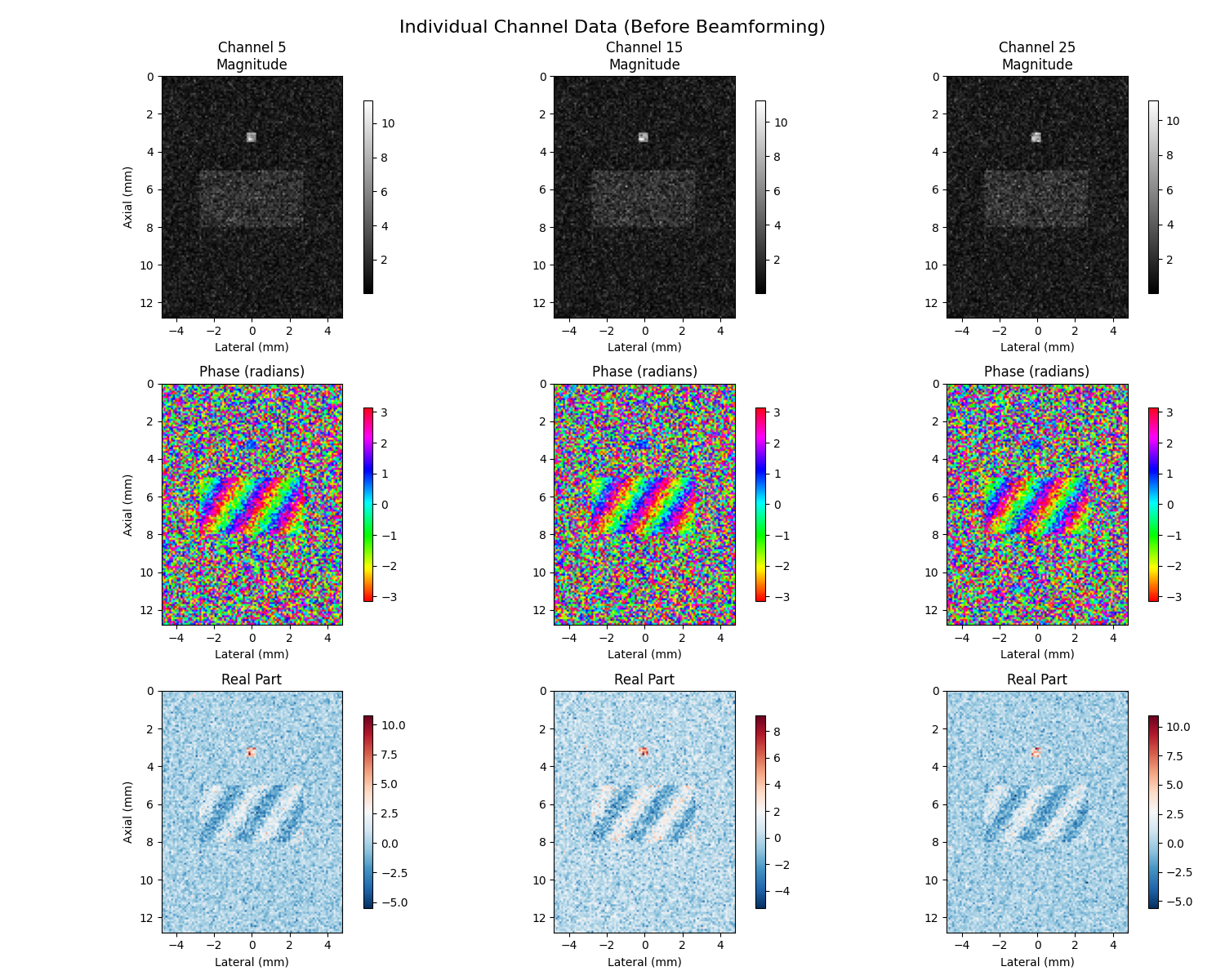
7. Individual Channel Visualization (Before Beamforming)

Individual channel visualization shows magnitude, phase, and real components before beamforming to understand signal relationships

# Select a few channels to visualize (channels 5, 15, 25)
channels_to_show = [5, 15, 25]
channel_labels = [f"Channel {ch}" for ch in channels_to_show]

# Use medium coherence data for demonstration
selected_beamsum = beamsum_medium

fig, axes = plt.subplots(3, len(channels_to_show), figsize=(15, 12))

for i, ch in enumerate(channels_to_show):
    channel_data = selected_beamsum[ch]  # Shape: (height, width)

    # Top row: Magnitude images
    magnitude = np.abs(channel_data)
    im1 = axes[0, i].imshow(magnitude, cmap="gray", extent=extent)
    axes[0, i].set_title(f"{channel_labels[i]}\nMagnitude")
    axes[0, i].set_xlabel("Lateral (mm)")
    if i == 0:
        axes[0, i].set_ylabel("Axial (mm)")
    plt.colorbar(im1, ax=axes[0, i], shrink=0.8)

    # Middle row: Phase images (using circular colormap)
    phase = np.angle(channel_data)
    im2 = axes[1, i].imshow(phase, cmap="hsv", vmin=-np.pi, vmax=np.pi, extent=extent)
    axes[1, i].set_title("Phase (radians)")
    axes[1, i].set_xlabel("Lateral (mm)")
    if i == 0:
        axes[1, i].set_ylabel("Axial (mm)")
    plt.colorbar(im2, ax=axes[1, i], shrink=0.8)

    # Bottom row: Real part
    real_part = np.real(channel_data)
    im3 = axes[2, i].imshow(real_part, cmap="RdBu_r", extent=extent)
    axes[2, i].set_title("Real Part")
    axes[2, i].set_xlabel("Lateral (mm)")
    if i == 0:
        axes[2, i].set_ylabel("Axial (mm)")
    plt.colorbar(im3, ax=axes[2, i], shrink=0.8)

plt.suptitle("Individual Channel Data (Before Beamforming)", fontsize=16)
plt.tight_layout()
plt.show()

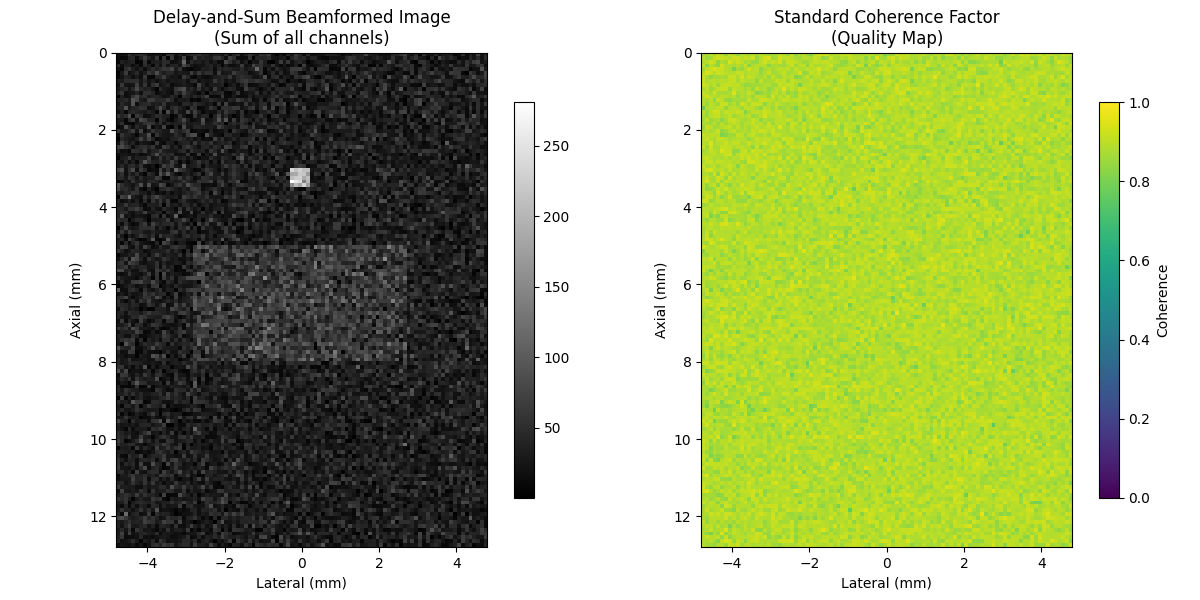
8. Delay-and-Sum Beamforming vs Coherence Factors

Compare DAS beamformed image with coherence quality map

# Compute delay-and-sum (DAS) beamformed image
das_image = np.sum(selected_beamsum, axis=0)
das_magnitude = np.abs(das_image)

# Compute standard coherence factor
cf_standard = coherence_factor(selected_beamsum, power_based=False)

fig, axes = plt.subplots(1, 2, figsize=(12, 6))

# DAS magnitude image
im1 = axes[0].imshow(das_magnitude, cmap="gray", extent=extent)
axes[0].set_title("Delay-and-Sum Beamformed Image\n(Sum of all channels)")
axes[0].set_xlabel("Lateral (mm)")
axes[0].set_ylabel("Axial (mm)")
plt.colorbar(im1, ax=axes[0], shrink=0.8)

# Coherence factor
im2 = axes[1].imshow(cf_standard, cmap="viridis", vmin=0, vmax=1, extent=extent)
axes[1].set_title("Standard Coherence Factor\n(Quality Map)")
axes[1].set_xlabel("Lateral (mm)")
axes[1].set_ylabel("Axial (mm)")
plt.colorbar(im2, ax=axes[1], shrink=0.8, label="Coherence")

plt.tight_layout()
plt.show()

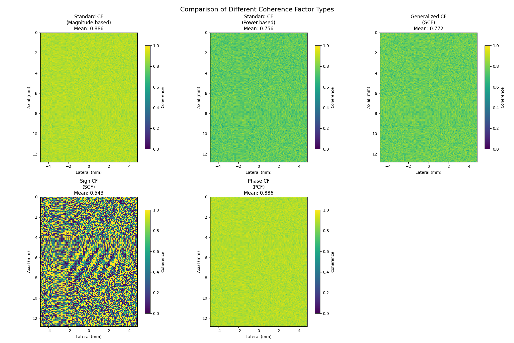
9. Comparison of Different Coherence Factor Types

Compare all coherence factor types: Standard, Generalized, Sign, and Phase

# Compute all coherence factor types
cf_magnitude = coherence_factor(selected_beamsum, power_based=False)
cf_power = coherence_factor(selected_beamsum, power_based=True)
gcf = generalized_coherence_factor(selected_beamsum)  # Optimal for diffuse scatterers
scf = sign_coherence_factor(selected_beamsum, power=1.0)
pcf = phase_coherence_factor(selected_beamsum, power=1.0)

# Create comparison visualization
coherence_types = [
    (cf_magnitude, "Standard CF\n(Magnitude-based)", "Standard coherence factor using magnitude ratios"),
    (cf_power, "Standard CF\n(Power-based)", "Power-based coherence factor (vbeam-compatible)"),
    (gcf, "Generalized CF\n(GCF)", "Uses spatial DFT for robustness in speckle regions"),
    (scf, "Sign CF\n(SCF)", "Uses only signal polarity - hardware efficient"),
    (pcf, "Phase CF\n(PCF)", "Based on phase coherence - amplitude independent"),
]

fig, axes = plt.subplots(2, 3, figsize=(18, 12))
axes = axes.flatten()

for i, (cf_data, title, _description) in enumerate(coherence_types):
    im = axes[i].imshow(cf_data, cmap="viridis", vmin=0, vmax=1, extent=extent)
    axes[i].set_title(f"{title}\nMean: {cf_data.mean():.3f}")
    axes[i].set_xlabel("Lateral (mm)")
    axes[i].set_ylabel("Axial (mm)")
    plt.colorbar(im, ax=axes[i], shrink=0.8, label="Coherence")

# Remove the last subplot (we only have 5 coherence types)
axes[5].remove()

plt.suptitle("Comparison of Different Coherence Factor Types", fontsize=16)
plt.tight_layout()
plt.show()

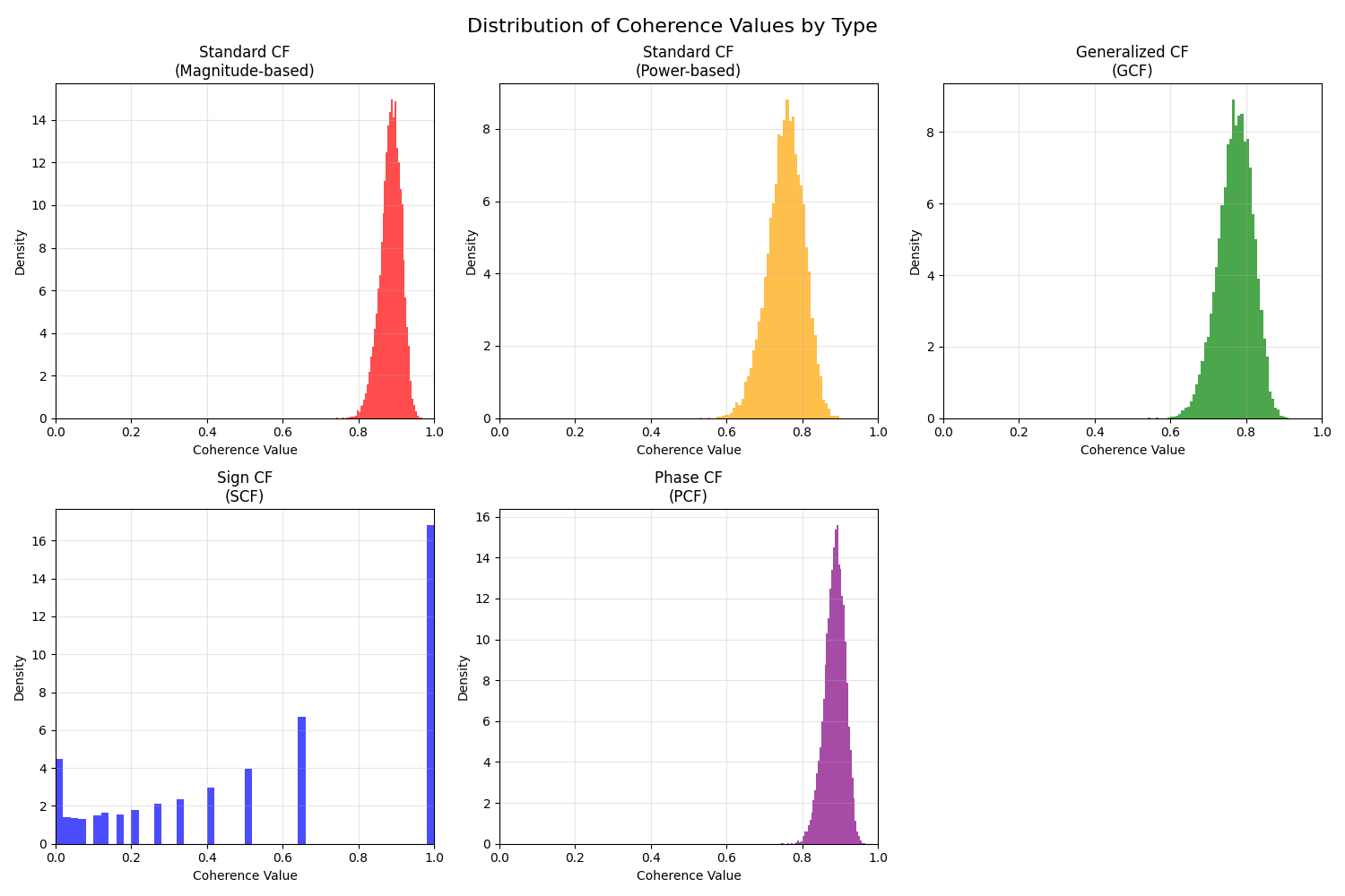
10. Quantitative Comparison of Coherence Factors

Quantitative comparison of coherence factor statistics

# Compute statistics for each coherence factor type
cf_stats = []
for cf_data, name, _ in coherence_types:
    stats = {
        "name": name,
        "mean": float(cf_data.mean()),
        "std": float(cf_data.std()),
        "min": float(cf_data.min()),
        "max": float(cf_data.max()),
        "median": float(np.median(cf_data)),
    }
    cf_stats.append(stats)


# Create histograms of coherence values
fig, axes = plt.subplots(2, 3, figsize=(15, 10))
axes = axes.flatten()

colors = ["red", "orange", "green", "blue", "purple"]
for i, ((cf_data, name, _), color) in enumerate(zip(coherence_types, colors)):
    axes[i].hist(cf_data.flatten(), bins=50, alpha=0.7, color=color, density=True)
    axes[i].set_xlabel("Coherence Value")
    axes[i].set_ylabel("Density")
    axes[i].set_title(name)
    axes[i].grid(True, alpha=0.3)
    axes[i].set_xlim(0, 1)

# Remove the last subplot
axes[5].remove()

plt.suptitle("Distribution of Coherence Values by Type", fontsize=16)
plt.tight_layout()
plt.show()

11. GCF Parameter M0 Analysis

Demonstrate the effect of the M0 parameter in Generalized Coherence Factor This is the spatial-frequency (i.e. field-of-view) cutoff for the GCF.

# Demonstrate the effect of different M0 values as discussed in Li & Li (2003)
# M0 controls the width of the low-frequency region used for GCF calculation
# Reduce to 3 values for cleaner 1x3 layout
m0_values = [0, 1, 2]
gcf_m0_results = []

for m0 in m0_values:
    try:
        gcf_m0 = generalized_coherence_factor(selected_beamsum, m0=m0)
        gcf_m0_results.append((gcf_m0, m0))
        mean_val = gcf_m0.mean()
        std_val = gcf_m0.std()
        print(f"   M0={m0}: Mean={mean_val:.3f}, Std={std_val:.3f}")
    except ValueError as e:
        print(f"   M0={m0}: {e}")
        gcf_m0_results.append((None, m0))

# Visualize different M0 values
fig, axes = plt.subplots(1, 3, figsize=(15, 5))

for i, (gcf_data, m0) in enumerate(gcf_m0_results):
    if gcf_data is not None:
        im = axes[i].imshow(gcf_data, cmap="viridis", vmin=0, vmax=1, extent=extent)
        axes[i].set_title(f"GCF with M0={m0}\nMean: {gcf_data.mean():.3f} ± {gcf_data.std():.3f}")
        axes[i].set_xlabel("Azimuth (mm)")
        axes[i].set_ylabel("Range (mm)")
        plt.colorbar(im, ax=axes[i], fraction=0.046, pad=0.04)
    else:
        axes[i].text(0.5, 0.5, f"M0={m0}\nInvalid", ha="center", va="center", transform=axes[i].transAxes, fontsize=14)
        axes[i].set_title(f"GCF with M0={m0} (Invalid)")
        axes[i].axis("off")

plt.suptitle(
    "Effect of GCF Cutoff Frequency M0\n"
    + "M0=0: Point targets only | M0=1: Optimal for diffuse scatterers | M0=2: More stable",
    fontsize=14,
)
plt.tight_layout()
plt.show()

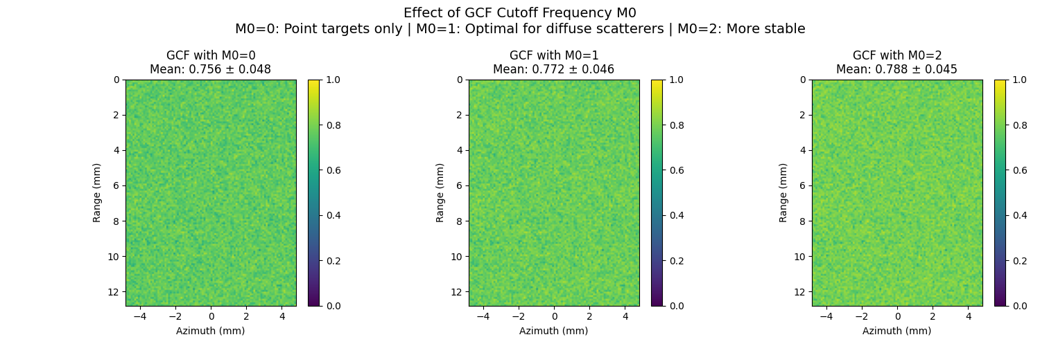
M0=0: Mean=0.756, Std=0.048
M0=1: Mean=0.772, Std=0.046
M0=2: Mean=0.788, Std=0.045

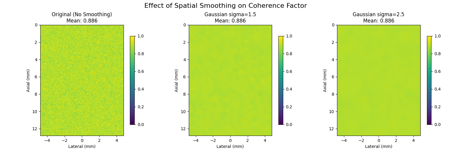
12. Spatial Smoothing Effect

Many methods, such as [2], smooth the coherence map to reduce noise before using it for aberration correction.

# Effect of spatial smoothing on coherence maps

# Apply different levels of spatial smoothing to standard coherence factor
cf_original = coherence_factor(selected_beamsum, power_based=False)

# Different smoothing kernel sizes - reduced to 3 for cleaner layout
smoothing_kernels = [1, 3, 5]  # in pixels
smoothed_cfs = []

for kernel_size in smoothing_kernels:
    if kernel_size == 1:
        # No smoothing
        smoothed_cf = cf_original
    else:
        # Gaussian smoothing
        smoothed_cf = ndimage.gaussian_filter(cf_original, sigma=kernel_size / 2)
    smoothed_cfs.append(smoothed_cf)

fig, axes = plt.subplots(1, 3, figsize=(15, 5))

for i, (smoothed_cf, kernel_size) in enumerate(zip(smoothed_cfs, smoothing_kernels)):
    im = axes[i].imshow(smoothed_cf, cmap="viridis", vmin=0, vmax=1, extent=extent)
    if kernel_size == 1:
        title = f"Original (No Smoothing)\nMean: {smoothed_cf.mean():.3f}"
    else:
        title = f"Gaussian sigma={kernel_size / 2:.1f}\nMean: {smoothed_cf.mean():.3f}"
    axes[i].set_title(title)
    axes[i].set_xlabel("Lateral (mm)")
    axes[i].set_ylabel("Axial (mm)")
    plt.colorbar(im, ax=axes[i], shrink=0.8)

plt.suptitle("Effect of Spatial Smoothing on Coherence Factor", fontsize=16)
plt.tight_layout()
plt.show()