Loading and Visualizing Ultrasound Images

This example demonstrates how to:

1. List available datasets

2. Download a PICMUS dataset using the public API

3. Visualize the beamformed ultrasound data

This serves as a minimal example of using the ultrasound_metrics.data module. The PICMUS (Plane-wave Imaging Challenge in Medical UltraSound) dataset [1] provides standardized ultrasound data for algorithm comparison.

References

[1]

H. Liebgott, A. Rodriguez-Molares, F. Cervenansky, J. A. Jensen and O. Bernard, “Plane-Wave Imaging Challenge in Medical Ultrasound,” 2016 IEEE International Ultrasonics Symposium (IUS), Tours, France, 2016, pp. 1-4, doi: 10.1109/ULTSYM.2016.7728908.

Example

1. Import required modules and functions

import matplotlib.pyplot as plt

from ultrasound_metrics.data import (
    create_bmode_image,
    db_zero,
    list_available_datasets,
)
from ultrasound_metrics.data.uff import (
    load_uff_dataset,
)

2. List available datasets

print("Available datasets:")
datasets = list_available_datasets()
for name, info in datasets.items():
    print(f"- {name}: {info['description']}")
print()

Available datasets:
- picmus_resolution_experiment: PICMUS challenge resolution/distortion test (experiment)
- picmus_contrast_experiment: PICMUS challenge contrast/speckle test (experiment)

3. Choose a dataset to visualize

dataset_name = "picmus_resolution_experiment"
print(f"Loading dataset: {dataset_name}")

Loading dataset: picmus_resolution_experiment

4. Load the dataset

beamformed_image, scan = load_uff_dataset(dataset_name)

print("Dataset loaded successfully!")
print(f"Data shape: {beamformed_image.shape}")
print(f"Data type: {beamformed_image.dtype}")
print(f"Data range: [{beamformed_image.min():.3f}, {beamformed_image.max():.3f}]")
print(f"Scan geometry: x={scan.x_axis.size}, z={scan.z_axis.size}")

Dataset loaded successfully!
Data shape: (387, 609)
Data type: complex64
Data range: [-56.675+21.870j, 52.407-5.226j]
Scan geometry: x=387, z=609

5. Convert to B-mode magnitude for visualization

data_array = create_bmode_image(beamformed_image)

print(f"After taking magnitude - Data range: [{data_array.min():.3f}, {data_array.max():.3f}]")

After taking magnitude - Data range: [0.003, 62.383]

6. Simple visualization with physical coordinates

fig, (ax1, ax2) = plt.subplots(1, 2, figsize=(12, 5))

# Get physical coordinates from scan geometry
x_coords = scan.x_axis
z_coords = scan.z_axis

# Plot the magnitude data with physical coordinates
# Use 'equal' aspect for square pixels, assuming isotropic grid spacing
im1 = ax1.imshow(
    data_array.T,
    cmap="gray",
    aspect="equal",
    extent=[x_coords.min(), x_coords.max(), z_coords.max(), z_coords.min()],
)
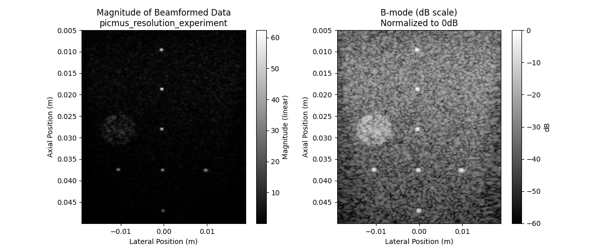
ax1.set_title(f"Magnitude of Beamformed Data\n{dataset_name}")
ax1.set_xlabel("Lateral Position (m)")
ax1.set_ylabel("Axial Position (m)")

# Add colorbar for linear magnitude image
fig.colorbar(im1, ax=ax1, orientation="vertical", label="Magnitude (linear)")

# Plot in dB scale (common for ultrasound visualization)
data_db = db_zero(data_array)

im2 = ax2.imshow(
    data_db.T,
    cmap="gray",
    aspect="equal",
    vmin=-60,
    vmax=0,
    extent=[x_coords.min(), x_coords.max(), z_coords.max(), z_coords.min()],
)
ax2.set_title("B-mode (dB scale)\nNormalized to 0dB")
ax2.set_xlabel("Lateral Position (m)")
ax2.set_ylabel("Axial Position (m)")

# Add colorbar for dB scale image
fig.colorbar(im2, ax=ax2, orientation="vertical", label="dB")

<matplotlib.colorbar.Colorbar object at 0x7f672ea007d0>

print("\nVisualization complete!")
print("Left: Raw beamformed data")
print("Right: B-mode in dB scale (typical ultrasound display)")
print("\nNote: This example demonstrates the new module structure:")
print("- General utilities (create_bmode_image, db_zero) from ultrasound_metrics.data")
print("- UFF-specific functionality (load_uff_dataset) from ultrasound_metrics.data.uff")

Visualization complete!
Left: Raw beamformed data
Right: B-mode in dB scale (typical ultrasound display)

Note: This example demonstrates the new module structure:
- General utilities (create_bmode_image, db_zero) from ultrasound_metrics.data
- UFF-specific functionality (load_uff_dataset) from ultrasound_metrics.data.uff