Tenengrad Sharpness Metric

This example uses a PICMUS dataset to demonstrate how to:

1. Compute and visualize the Tenengrad sharpness metric [1]

2. Compare sharpness between datasets with different characteristics

3. Show how the metric responds to different ROI selections

[2] uses the Tenengrad sharpness metric to compare the lateral focusing quality across different speed-of-sound profiles.

References

[1]

Groen, F. C., Young, I. T., & Ligthart, G. (1985). A comparison of different focus functions for use in autrasound algorithms. Cytometry, 6(2), 81-91.

[2] (1,2)

Vrålstad, A.E. et al. (2024). Coherence Based Sound Speed Aberration Correction — with clinical validation in fetal ultrasound. arXiv:2411.16551

Example

1. Import required modules and functions

import matplotlib.pyplot as plt
import numpy as np

from ultrasound_metrics.data.uff import load_uff_dataset
from ultrasound_metrics.data.visualize_bmode import db_zero
from ultrasound_metrics.metrics.sharpness import tenengrad
from ultrasound_metrics.roi.masks import build_mask

2. Load PICMUS datasets

image_resolution, scan_resolution = load_uff_dataset("picmus_resolution_experiment")
image_resolution = image_resolution.T

image_contrast, scan_contrast = load_uff_dataset("picmus_contrast_experiment")
image_contrast = image_contrast.T

print(f"Resolution/distortion dataset image shape: {image_resolution.shape}")
print(f"Contrast/speckle dataset image shape: {image_contrast.shape}")

Resolution/distortion dataset image shape: (609, 387)
Contrast/speckle dataset image shape: (609, 387)

3. Calculate edge-enhanced image

This is an intermediate step for Tenengrad sharpness.

sharpness_img_resolution = tenengrad(image_resolution, reduce_sum=False)
print("sharpness image shape:", sharpness_img_resolution.shape, "(resolution/distortion dataset)")

sharpness_img_contrast = tenengrad(image_contrast, reduce_sum=False)
print("sharpness image shape:", sharpness_img_contrast.shape, "(contrast/speckle dataset)")

sharpness image shape: (609, 387) (resolution/distortion dataset)
sharpness image shape: (609, 387) (contrast/speckle dataset)

4. Visualize the original images and their sharpness maps

fig, axes = plt.subplots(2, 3, figsize=(15, 10), gridspec_kw={"width_ratios": [1, 1, 1]})

# Share x and y axes for the histogram plots (right column)
axes[0, 2].sharex(axes[1, 2])
axes[0, 2].sharey(axes[1, 2])

# Get coordinate arrays for proper axis labeling
x_coords_res = scan_resolution.x_axis
z_coords_res = scan_resolution.z_axis
x_coords_con = scan_contrast.x_axis
z_coords_con = scan_contrast.z_axis

# Define common visualization parameters
vmin = -60  # dB range for B-mode images
vmax = 0
sharpness_vmin = 0
sharpness_vmax = 2

# Row 1: Resolution/distortion dataset
extent_res = [x_coords_res.min(), x_coords_res.max(), z_coords_res.max(), z_coords_res.min()]
im1 = axes[0, 0].imshow(db_zero(image_resolution), cmap="gray", vmin=vmin, vmax=vmax, extent=extent_res)
axes[0, 0].set_title("B-mode (dB)\n(Resolution/distortion dataset)")
axes[0, 0].set_xlabel("Lateral Position (m)")
axes[0, 0].set_ylabel("Axial Position (m)")

im2 = axes[0, 1].imshow(
    sharpness_img_resolution, cmap="hot", extent=extent_res, vmin=sharpness_vmin, vmax=sharpness_vmax
)
axes[0, 1].set_title("Tenengrad Sharpness Image\n(Resolution/distortion dataset)")
axes[0, 1].set_xlabel("Lateral Position (m)")
axes[0, 1].set_ylabel("Axial Position (m)")

# Histogram of sharpness values for resolution/distortion dataset
axes[0, 2].hist(sharpness_img_resolution.flatten(), bins=50, alpha=0.7, color="red")
axes[0, 2].set_title("Sharpness Value Distribution\n(Resolution/distortion dataset)")
axes[0, 2].set_xlabel("Sharpness Value")
axes[0, 2].set_ylabel("Frequency")
axes[0, 2].set_yscale("log")

# Row 2: Contrast/speckle dataset
extent_con = [x_coords_con.min(), x_coords_con.max(), z_coords_con.max(), z_coords_con.min()]
im3 = axes[1, 0].imshow(db_zero(image_contrast), cmap="gray", vmin=vmin, vmax=vmax, extent=extent_con)
axes[1, 0].set_title("B-mode (dB)\n(Contrast/speckle dataset)")
axes[1, 0].set_xlabel("Lateral Position (m)")
axes[1, 0].set_ylabel("Axial Position (m)")

im4 = axes[1, 1].imshow(sharpness_img_contrast, cmap="hot", extent=extent_con, vmin=sharpness_vmin, vmax=sharpness_vmax)
axes[1, 1].set_title("Tenengrad Sharpness Image\n(Contrast/speckle dataset)")
axes[1, 1].set_xlabel("Lateral Position (m)")
axes[1, 1].set_ylabel("Axial Position (m)")

# Histogram of sharpness values for contrast experiment
axes[1, 2].hist(sharpness_img_contrast.flatten(), bins=50, alpha=0.7, color="blue")
axes[1, 2].set_title("Sharpness Value Distribution\n(Contrast/speckle dataset)")
axes[1, 2].set_xlabel("Sharpness Value")
axes[1, 2].set_ylabel("Frequency")
axes[1, 2].set_yscale("log")

# Add colorbars
plt.colorbar(im1, ax=axes[0, 0], label="dB")
plt.colorbar(im3, ax=axes[1, 0], label="dB")
plt.colorbar(im2, ax=axes[0, 1], label="Lateral Sharpness")
plt.colorbar(im4, ax=axes[1, 1], label="Lateral Sharpness")

plt.tight_layout()
plt.show()

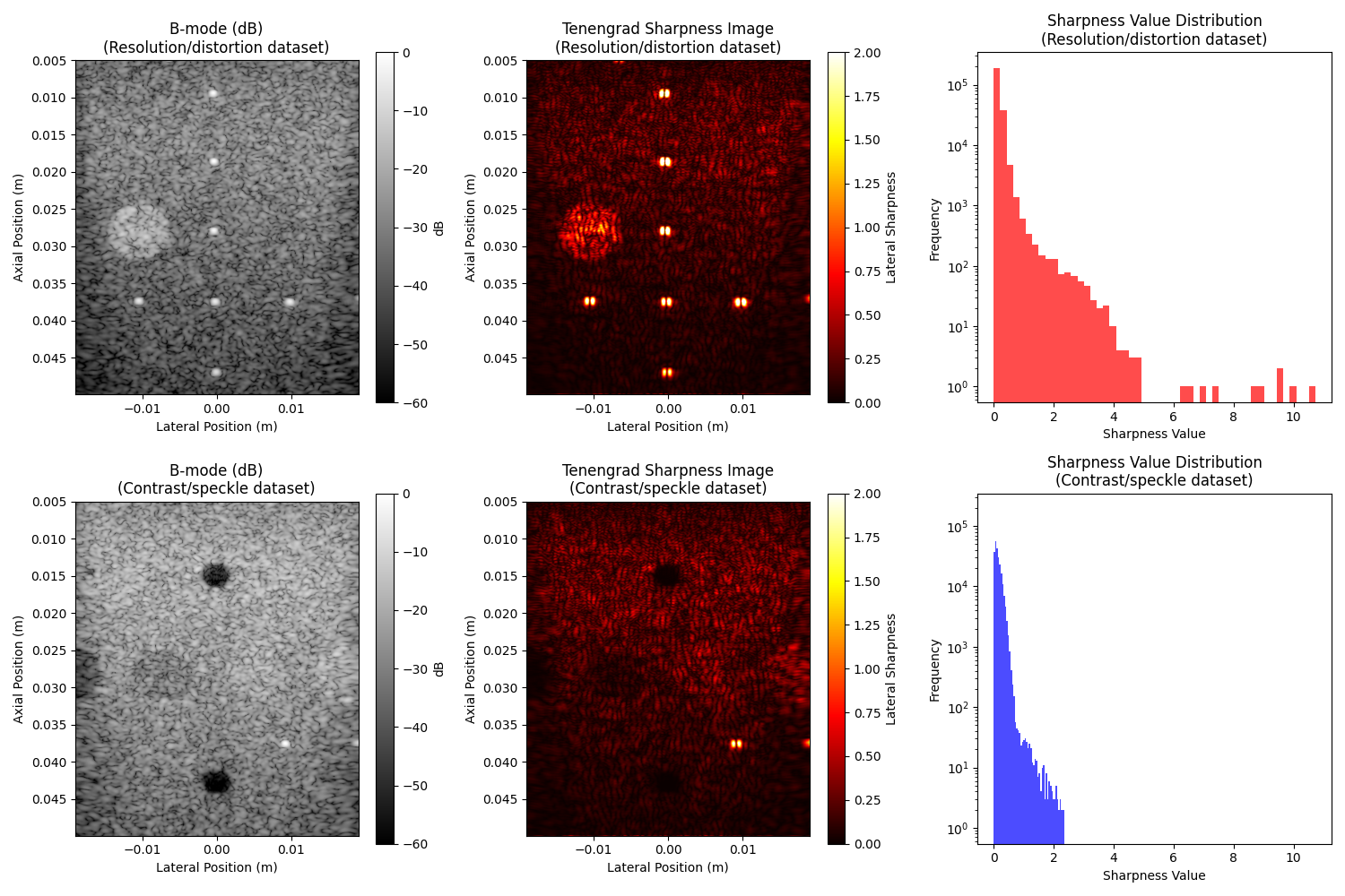
5. Calculate overall sharpness metrics for both datasets

print("\n=== Overall Tenengrad Sharpness Comparison ===")

# Calculate total sharpness (sum) and normalized sharpness (mean)
sharpness_resolution = tenengrad(image_resolution, normalize=False)
sharpness_normalized_resolution = tenengrad(image_resolution, normalize=True)

sharpness_contrast = tenengrad(image_contrast, normalize=False)
sharpness_normalized_contrast = tenengrad(image_contrast, normalize=True)

print("Resolution experiment:")
print(f"  Total sharpness: {float(sharpness_resolution):.1f}")
print(f"  Normalized sharpness: {float(sharpness_normalized_resolution):.4f}")

print("\nContrast experiment:")
print(f"  Total sharpness: {float(sharpness_contrast):.1f}")
print(f"  Normalized sharpness: {float(sharpness_normalized_contrast):.4f}")

# Calculate ratio
ratio = float(sharpness_normalized_resolution) / float(sharpness_normalized_contrast)
print(f"\nSharpness ratio (Resolution/Contrast): {ratio:.2f}")

if ratio > 1.2:
    print("✅ Resolution/distortion dataset shows higher sharpness as expected!")
    print("   Point targets create sharper edges than diffuse lesions.")
elif ratio > 0.8:
    print("️Similar overall sharpness between datasets.")
else:
    print("⚠️  Contrast/speckle dataset shows higher sharpness.")

=== Overall Tenengrad Sharpness Comparison ===
Resolution experiment:
  Total sharpness: 35788.9
  Normalized sharpness: 0.1519

Contrast experiment:
  Total sharpness: 35172.2
  Normalized sharpness: 0.1492

Sharpness ratio (Resolution/Contrast): 1.02
️Similar overall sharpness between datasets.

6. Compare sharpness across regions

We should expect that the point target region is sharper than the background speckle region. Here, we visualize the sharpness in different regions and validate this expectation.

# For the resolution experiment, create ROIs around different areas
center_target = (0.000, 0.0275)  # Center of a point target (x, z in meters)
center_background = (0.015, 0.0275)  # Background speckle region

# Create circular ROIs
target_radius = 0.003  # 3mm radius
background_radius = 0.005  # 5mm radius

# Build masks for the resolution experiment
mask_target = build_mask(
    position=center_target,
    dimension=target_radius,
    x_axis=scan_resolution.x_axis,
    z_axis=scan_resolution.z_axis,
    shape="circle",
)

mask_background = build_mask(
    position=center_background,
    dimension=background_radius,
    x_axis=scan_resolution.x_axis,
    z_axis=scan_resolution.z_axis,
    shape="circle",
)

fig, axes = plt.subplots(1, 3, figsize=(15, 5))

# Show original image with ROI overlays
extent = [x_coords_res.min(), x_coords_res.max(), z_coords_res.max(), z_coords_res.min()]

# Original image
im1 = axes[0].imshow(db_zero(image_resolution), cmap="gray", vmin=vmin, vmax=vmax, extent=extent)
axes[0].contour(
    np.linspace(extent[0], extent[1], mask_target.shape[1]),
    np.linspace(extent[3], extent[2], mask_target.shape[0]),
    mask_target,
    colors="red",
    linewidths=2,
)
axes[0].contour(
    np.linspace(extent[0], extent[1], mask_background.shape[1]),
    np.linspace(extent[3], extent[2], mask_background.shape[0]),
    mask_background,
    colors="blue",
    linewidths=2,
)
axes[0].set_title("B-mode with ROIs\n(Red: Target, Blue: Background)")
axes[0].set_xlabel("Lateral Position (m)")
axes[0].set_ylabel("Axial Position (m)")

# Calculate sharpness in different ROIs
sharpness_target = tenengrad(image_resolution, roi=mask_target, normalize=True)
sharpness_background = tenengrad(image_resolution, roi=mask_background, normalize=True)

# Target ROI
masked_target = np.ma.masked_where(~mask_target, sharpness_img_resolution)
im2 = axes[1].imshow(masked_target, cmap="hot", extent=extent, vmin=sharpness_vmin, vmax=sharpness_vmax)
axes[1].set_title(f"Target ROI Sharpness\nMean: {float(sharpness_target):.4f}")
axes[1].set_xlabel("Lateral Position (m)")
axes[1].set_ylabel("Axial Position (m)")

# Background ROI
masked_background = np.ma.masked_where(~mask_background, sharpness_img_resolution)
im3 = axes[2].imshow(masked_background, cmap="hot", extent=extent, vmin=sharpness_vmin, vmax=sharpness_vmax)
axes[2].set_title(f"Background ROI Sharpness\nMean: {float(sharpness_background):.4f}")
axes[2].set_xlabel("Lateral Position (m)")
axes[2].set_ylabel("Axial Position (m)")

# Add colorbars
plt.colorbar(im1, ax=axes[0], label="dB")
plt.colorbar(im2, ax=axes[1], label="Lateral Sharpness")
plt.colorbar(im3, ax=axes[2], label="Lateral Sharpness")

plt.tight_layout()
plt.show()

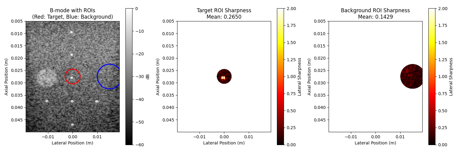
7. Compare sharpness across regions

We should expect that the point target region is sharper than the background speckle region.

print("\n=== ROI-based Sharpness Analysis ===")
print(f"Point target region sharpness: {float(sharpness_target):.4f}")
print(f"Background speckle sharpness: {float(sharpness_background):.4f}")

target_bg_ratio = float(sharpness_target) / float(sharpness_background)
print(f"Target/Background ratio: {target_bg_ratio:.2f}")

if target_bg_ratio > 1.5:
    print("✅ Point target region is significantly sharper than background!")
    print("   This demonstrates the metric's sensitivity to small structures.")

=== ROI-based Sharpness Analysis ===
Point target region sharpness: 0.2650
Background speckle sharpness: 0.1429
Target/Background ratio: 1.85
✅ Point target region is significantly sharper than background!
   This demonstrates the metric's sensitivity to small structures.

8. Summary

We have shown that the Tenengrad sharpness metric can be used to compare the sharpness of different regions in an image.

This metric can be valuable for [2]:

• Assessing ultrasound image focusing quality

• Comparing different imaging parameters or techniques

• Automated quality control in ultrasound systems