Contrast Metric for Calibrated Phantoms

This example demonstrates contrast measurement using a calibrated CIRS 040GSE phantom, which is helpful for validating beamforming algorithms against known specifications.

Mathematical Definition

The contrast between two regions (denoted inside \(i\) and outside \(o\)) is defined as:

\[C = \frac{\mu_i}{\mu_o}\]

where:

\[\mu_i = \mathbb{E}\left\{|s_i|^2\right\}\]

\[\mu_o = \mathbb{E}\left\{|s_o|^2\right\}\]

are, respectively, the mean signal power inside and outside the lesion, where \(s\) denotes the signal. Contrast can take any positive real value, and \(C \to \infty\) as \(\mu_o \to 0\).

Contrast is often expressed in decibels as:

\[C[\text{dB}] = 10\log_{10} C\]

When to use contrast:

• Calibrated phantoms with known lesion contrast levels

• Linear imaging where intensity directly relates to scattering strength

• Validation against manufacturer specifications

When to use alternatives:

• gcnr() for nonlinear imaging methods (e.g., coherence-based beamforming)

• cnr() when accounting for noise statistics is important

• Dynamic range compression affects traditional contrast measurements

This example uses the contrast metric as described in [1] and demonstrates analysis using the PICMUS dataset [2].

References

[1]

A. Rodriguez-Molares, O. M. Hoel Rindal, J. D’hooge, S. -E. Måsøy, A. Austeng and H. Torp, “The Generalized Contrast-to-Noise Ratio,” 2018 IEEE International Ultrasonics Symposium (IUS), Kobe, Japan, 2018, pp. 1-4, doi: 10.1109/ULTSYM.2018.8580101.

[2]

H. Liebgott, A. Rodriguez-Molares, F. Cervenansky, J. A. Jensen and O. Bernard, “Plane-Wave Imaging Challenge in Medical Ultrasound,” 2016 IEEE International Ultrasonics Symposium (IUS), Tours, France, 2016, pp. 1-4, doi: 10.1109/ULTSYM.2016.7728908.

Example

import matplotlib.colors as mcolors
import matplotlib.pyplot as plt
import numpy as np
import pandas as pd
from matplotlib.patches import Patch

from ultrasound_metrics.data import db_zero
from ultrasound_metrics.data.uff import load_uff_dataset
from ultrasound_metrics.metrics.contrast import contrast
from ultrasound_metrics.roi.masks import build_mask

Load the ultrasound dataset

# Load the PICMUS contrast/speckle dataset which contains lesions with known contrast levels
dataset_name = "picmus_contrast_experiment"
image, scan = load_uff_dataset(dataset_name)
image = image.T
extent = (scan.x_axis.min(), scan.x_axis.max(), scan.z_axis.max(), scan.z_axis.min())

Downloading PICMUS_experiment_contrast_speckle.uff:   0%|          | 0.00/146M [00:00<?, ?B/s]
Downloading PICMUS_experiment_contrast_speckle.uff:   1%|          | 1.05M/146M [00:00<00:29, 4.86MB/s]
Downloading PICMUS_experiment_contrast_speckle.uff:   5%|▌         | 7.34M/146M [00:00<00:05, 27.3MB/s]
Downloading PICMUS_experiment_contrast_speckle.uff:  12%|█▏        | 16.8M/146M [00:00<00:02, 50.6MB/s]
Downloading PICMUS_experiment_contrast_speckle.uff:  18%|█▊        | 26.2M/146M [00:00<00:01, 63.0MB/s]
Downloading PICMUS_experiment_contrast_speckle.uff:  25%|██▌       | 36.7M/146M [00:00<00:01, 74.8MB/s]
Downloading PICMUS_experiment_contrast_speckle.uff:  32%|███▏      | 47.2M/146M [00:00<00:01, 78.5MB/s]
Downloading PICMUS_experiment_contrast_speckle.uff:  40%|███▉      | 57.7M/146M [00:00<00:01, 85.6MB/s]
Downloading PICMUS_experiment_contrast_speckle.uff:  46%|████▌     | 67.1M/146M [00:00<00:00, 84.4MB/s]
Downloading PICMUS_experiment_contrast_speckle.uff:  53%|█████▎    | 76.5M/146M [00:01<00:00, 86.8MB/s]
Downloading PICMUS_experiment_contrast_speckle.uff:  59%|█████▉    | 86.0M/146M [00:01<00:00, 86.3MB/s]
Downloading PICMUS_experiment_contrast_speckle.uff:  66%|██████▋   | 96.5M/146M [00:01<00:00, 91.4MB/s]
Downloading PICMUS_experiment_contrast_speckle.uff:  73%|███████▎  | 106M/146M [00:01<00:00, 88.4MB/s]
Downloading PICMUS_experiment_contrast_speckle.uff:  79%|███████▉  | 115M/146M [00:01<00:00, 86.4MB/s]
Downloading PICMUS_experiment_contrast_speckle.uff:  86%|████████▌ | 125M/146M [00:01<00:00, 81.7MB/s]
Downloading PICMUS_experiment_contrast_speckle.uff:  92%|█████████▏| 133M/146M [00:01<00:00, 79.9MB/s]
Downloading PICMUS_experiment_contrast_speckle.uff:  97%|█████████▋| 142M/146M [00:01<00:00, 79.0MB/s]
Downloading PICMUS_experiment_contrast_speckle.uff: 100%|██████████| 146M/146M [00:01<00:00, 75.8MB/s]

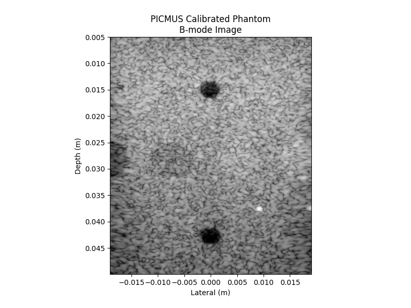
Visualize the B-mode image

image_db = db_zero(image)
fig, ax = plt.subplots(figsize=(8, 6))
ax.imshow(image_db, cmap="gray", extent=extent, vmin=-60, vmax=0)
ax.set_title("PICMUS Calibrated Phantom\nB-mode Image")
ax.set_xlabel("Lateral (m)")
_ = ax.set_ylabel("Depth (m)")

Define known lesion locations based on PICMUS phantom geometry

Define lesion locations and compute contrast PICMUS phantom specifications: 8mm diameter (4mm radius) lesions at -3dB and +3dB contrast

lesion_specs = [
    {"name": "-3dB lesion", "center": (-0.007, 0.028), "expected_contrast_db": -3},
    {"name": "+3dB lesion", "center": (0.0055, 0.028), "expected_contrast_db": +3},
]

# https://www.cirsinc.com/wp-content/uploads/2019/04/040GSE-DS-120418.pdf
lesion_radius = 0.004
# include the background region, but don't include other lesions
background_radius = lesion_radius * 2

Compute contrast for each lesion ROI

results_data = []
for spec in lesion_specs:
    center = spec["center"]

    mask_lesion = build_mask(center, lesion_radius, scan.x_axis, scan.z_axis, "circle")
    mask_background_and_lesion = build_mask(center, background_radius, scan.x_axis, scan.z_axis, "circle")
    mask_background = mask_background_and_lesion & ~mask_lesion

    # Compute contrast between lesion and background regions
    measured_db = contrast(image[mask_lesion], image[mask_background], db=True)
    error_db = measured_db - spec["expected_contrast_db"]

    results_data.append({
        "Lesion": spec["name"],
        "Expected (dB)": spec["expected_contrast_db"],
        "Measured (dB)": measured_db,
        "Error (dB)": error_db,
        "mask_lesion": mask_lesion,
        "mask_background": mask_background,
    })

Display results table

results_df = pd.DataFrame(results_data)
print("=== Contrast Measurement Results ===")
print(results_df[["Lesion", "Expected (dB)", "Measured (dB)", "Error (dB)"]].round(2))

# Summary statistics
errors = results_df["Error (dB)"].values
print(f"\nMean absolute error: {np.mean(np.abs(errors)):.2f} dB")
print(f"RMS error: {np.sqrt(np.mean(errors**2)):.2f} dB")

=== Contrast Measurement Results ===
        Lesion  Expected (dB)  Measured (dB)  Error (dB)
0  -3dB lesion             -3          -3.44       -0.44
1  +3dB lesion              3           2.20       -0.80

Mean absolute error: 0.62 dB
RMS error: 0.65 dB

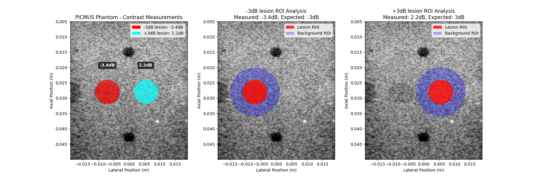
The contrast measurements are close but slightly more negative than expected. The phantom might not be perfectly calibrated.

Visualize ROIs and measurements

fig, axes = plt.subplots(1, 1 + len(results_df), figsize=(18, 6))

# First subplot: Overview with all lesions
ax1 = axes[0]
ax1.imshow(image_db, cmap="gray", extent=extent, vmin=-60, vmax=0)
colors = ["red", "cyan"]
legend_elements = []

for i, (_, row) in enumerate(results_df.iterrows()):
    # Overlay lesion ROI
    lesion_overlay = np.ma.masked_where(~row["mask_lesion"], np.ones_like(image_db))
    ax1.imshow(lesion_overlay, alpha=0.7, extent=extent, cmap=mcolors.ListedColormap([colors[i]]))

    # Add measurement labels
    center = lesion_specs[i]["center"]
    ax1.text(
        center[0],
        center[1] - 0.008,
        f"{row['Measured (dB)']:.1f}dB",
        ha="center",
        va="bottom",
        color="white",
        fontweight="bold",
        bbox={"boxstyle": "round,pad=0.3", "facecolor": "black", "alpha": 0.7},
    )

    legend_elements.append(Patch(facecolor=colors[i], label=f"{row['Lesion']}: {row['Measured (dB)']:.1f}dB"))

ax1.set_title("PICMUS Phantom - Contrast Measurements")
ax1.set_xlabel("Lateral Position (m)")
ax1.set_ylabel("Axial Position (m)")
ax1.legend(handles=legend_elements, loc="upper right")

# Individual lesion subplots: Show each lesion with its background ROI
for i, (_, row) in enumerate(results_df.iterrows()):
    ax = axes[i + 1]
    ax.imshow(image_db, cmap="gray", extent=extent, vmin=-60, vmax=0)

    # Show lesion (red) and background (blue) ROIs
    lesion_overlay = np.ma.masked_where(~row["mask_lesion"], np.ones_like(image_db))
    bg_overlay = np.ma.masked_where(~row["mask_background"], np.ones_like(image_db))

    ax.imshow(lesion_overlay, alpha=0.8, extent=extent, cmap=mcolors.ListedColormap(["red"]))
    ax.imshow(bg_overlay, alpha=0.3, extent=extent, cmap=mcolors.ListedColormap(["blue"]))

    ax.set_title(
        f"{row['Lesion']} ROI Analysis\nMeasured: {row['Measured (dB)']:.1f}dB, Expected: {row['Expected (dB)']}dB"
    )
    ax.set_xlabel("Lateral Position (m)")
    ax.set_ylabel("Axial Position (m)")

    roi_legend = [
        Patch(facecolor="red", alpha=0.8, label="Lesion ROI"),
        Patch(facecolor="blue", alpha=0.3, label="Background ROI"),
    ]
    ax.legend(handles=roi_legend, loc="upper right")

Show all figures (if run as a script)

plt.show()