Generalized Contrast-to-Noise Ratio (gCNR) Metric

This example demonstrates how to:

1. Load an ultrasound dataset

2. Choose ROI selection mode (interactive or hardcoded)

3. Visualize the B-mode image and select signal/noise ROIs

4. Print ROI summary and statistics

5. Compute and print the gCNR (optionally plot PDFs)

This workflow is backend-agnostic and uses the helper functions from ultrasound_metrics. The gCNR metric follows the formulation in [1] and uses the PICMUS dataset [2].

References

[1]

A. Rodriguez-Molares, O. M. Hoel Rindal, J. D’hooge, S. -E. Måsøy, A. Austeng and H. Torp, “The Generalized Contrast-to-Noise Ratio,” 2018 IEEE International Ultrasonics Symposium (IUS), Kobe, Japan, 2018, pp. 1-4, doi: 10.1109/ULTSYM.2018.8580101.

[2]

H. Liebgott, A. Rodriguez-Molares, F. Cervenansky, J. A. Jensen and O. Bernard, “Plane-Wave Imaging Challenge in Medical Ultrasound,” 2016 IEEE International Ultrasonics Symposium (IUS), Tours, France, 2016, pp. 1-4, doi: 10.1109/ULTSYM.2016.7728908.

Example

1. Import required modules and functions

import matplotlib.pyplot as plt
import numpy as np

from ultrasound_metrics.data import db_zero

# (Optional) for interactive ROI selection
from ultrasound_metrics.interactive.napari_utils import load_ultrasound_for_napari, select_rois_with_labels
from ultrasound_metrics.metrics.gcnr import gcnr
from ultrasound_metrics.roi.masks import build_mask

2. Set ROI selection mode

def is_headless_environment():
    """Detect if running in headless environment (no GUI available)."""
    import os
    import sys

    # Check for ReadTheDocs
    if os.environ.get("READTHEDOCS") == "True":
        return True

    # Check for sphinx-gallery module
    return "sphinx_gallery" in sys.modules


# Interactive if not headless (feel free to change to True / False for local testing)
use_interactive = not is_headless_environment()

3. Load the ultrasound dataset

image_data, metadata, scan = load_ultrasound_for_napari("picmus_resolution_experiment")

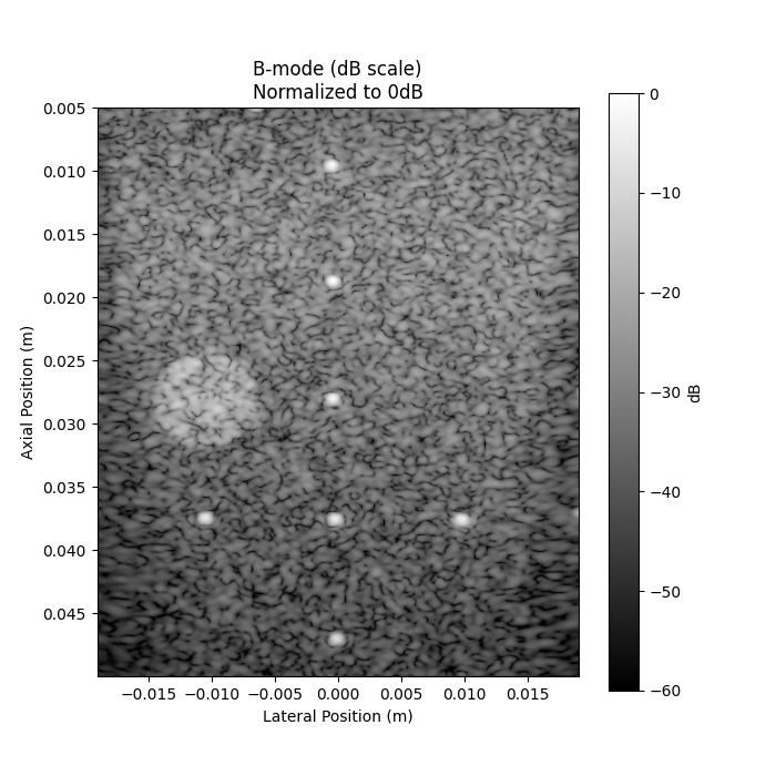
4. Visualize the B-mode image to help select ROI center and radii

x_coords = metadata["x_axis"]
z_coords = metadata["z_axis"]

# Only convert to dB if not already in dB scale
if metadata.get("use_db_scale", True):
    image_db = image_data
else:
    image_db = db_zero(image_data)

if not use_interactive:
    plt.figure(figsize=(7, 7))
    plt.imshow(
        image_db,
        cmap="gray",
        aspect="equal",
        vmin=-60,
        vmax=0,
        extent=[x_coords.min(), x_coords.max(), z_coords.max(), z_coords.min()],
    )
    plt.title("B-mode (dB scale)\nNormalized to 0dB")
    plt.xlabel("Lateral Position (m)")
    plt.ylabel("Axial Position (m)")
    plt.colorbar(label="dB")
    plt.show()

5. Select ROIs (either interactively or with hardcoded masks)

if use_interactive:
    roi_result = select_rois_with_labels(image=image_data)
    mask_signal = roi_result["mask_signal"]
    mask_noise = roi_result["mask_noise"]
else:
    # Hardcoded ROI selection and visualization
    center = (-0.0105, 0.028)  # (x, z) in meters
    signal_radius = 0.004  # 4 mm
    noise_radius = 0.0075  # 7.5 mm
    mask_signal = build_mask(
        position=center, dimension=signal_radius, x_axis=metadata["x_axis"], z_axis=metadata["z_axis"], shape="circle"
    )
    mask_noise_outer = build_mask(
        position=center, dimension=noise_radius, x_axis=metadata["x_axis"], z_axis=metadata["z_axis"], shape="circle"
    )
    mask_noise = np.logical_and(mask_noise_outer, ~mask_signal)
    # --- Visualization of B-mode, signal, and noise masks ---
    fig, axs = plt.subplots(1, 3, figsize=(15, 5))
    bmode_args = {
        "extent": [x_coords.min(), x_coords.max(), z_coords.max(), z_coords.min()],
        "cmap": "gray",
        "vmin": -60,
        "vmax": 0,
    }
    im0 = axs[0].imshow(image_db, **bmode_args)
    axs[0].set_title("B-mode (dB)")
    axs[0].set_xlabel("Lateral (m)")
    axs[0].set_ylabel("Axial (m)")
    fig.colorbar(im0, ax=axs[0], orientation="vertical", label="dB")
    masked_signal = np.ma.masked_where(~mask_signal, image_db)
    im1 = axs[1].imshow(masked_signal, **bmode_args)
    axs[1].set_title("Signal ROI")
    axs[1].set_xlabel("Lateral (m)")
    axs[1].set_ylabel("Axial (m)")
    fig.colorbar(im1, ax=axs[1], orientation="vertical", label="dB")
    masked_noise = np.ma.masked_where(~mask_noise, image_db)
    im2 = axs[2].imshow(masked_noise, **bmode_args)
    axs[2].set_title("Noise ROI")
    axs[2].set_xlabel("Lateral (m)")
    axs[2].set_ylabel("Axial (m)")
    fig.colorbar(im2, ax=axs[2], orientation="vertical", label="dB")
    plt.tight_layout()
    plt.show()

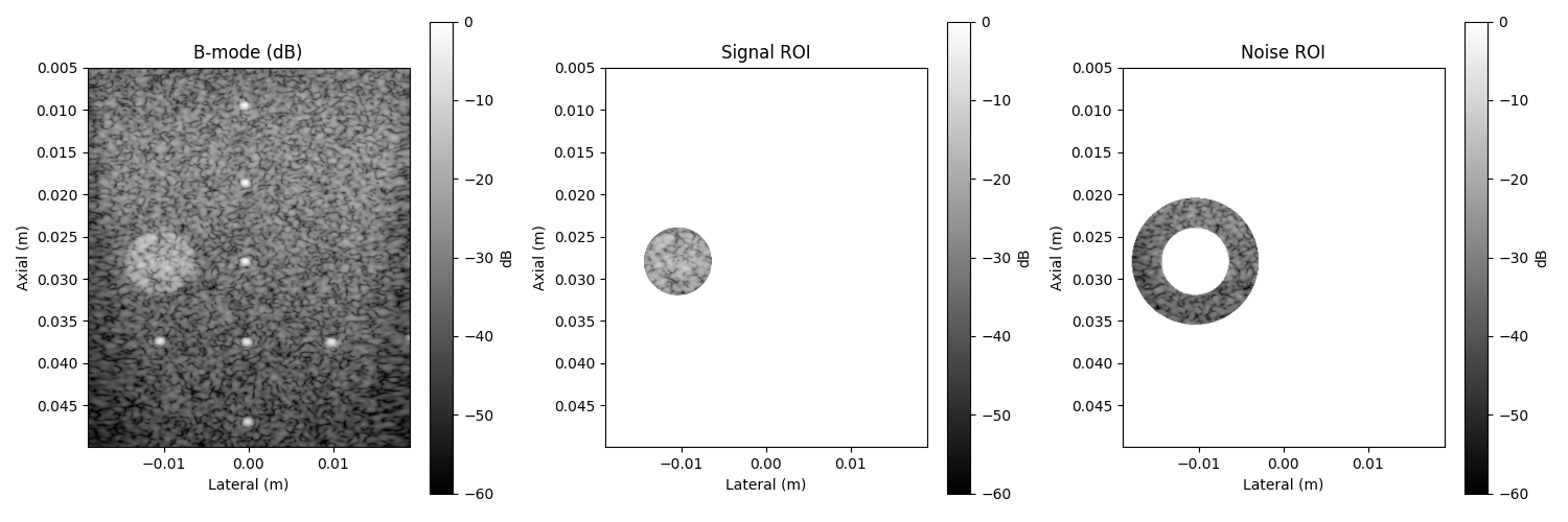
6. Print ROI summary

signal_pixels = mask_signal.sum()
noise_pixels = mask_noise.sum()
print("\n=== ROI Selection Summary ===")
print(f"Signal region pixel count: {signal_pixels}")
print(f"Noise region pixel count: {noise_pixels}")

=== ROI Selection Summary ===
Signal region pixel count: 6895
Noise region pixel count: 17361

7. Print basic statistics

values_signal = image_data[mask_signal]
values_noise = image_data[mask_noise]
print("\n=== Region Statistics ===")
print(f"Signal mean: {values_signal.mean():.3f} dB")
print(f"Noise mean: {values_noise.mean():.3f} dB")

=== Region Statistics ===
Signal mean: -23.187 dB
Noise mean: -35.079 dB

8. Compute and print gCNR (optionally plot PDFs)

fig, ax = plt.subplots(figsize=(6, 4))
gcnr_value = gcnr(values_inside=values_signal, values_outside=values_noise, ax=ax)
plt.tight_layout()
plt.show()

print("\n=== gCNR Results ===")
print(f"gCNR: {gcnr_value:.3f}")

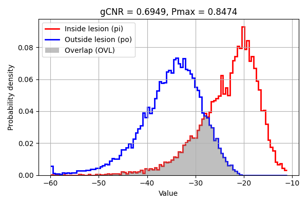
=== gCNR Results ===
gCNR: 0.695