Signal-to-Noise Ratio (SNR) for Speckle Regions

This example demonstrates the Signal-to-Noise Ratio (SNR) metric for ultrasound speckle analysis. We explore how SNR varies in different tissue regions and validate measurements against theoretical Rayleigh distribution values.

Mathematical Definition

The Signal-to-Noise Ratio for ultrasound speckle is defined as the ratio of mean to standard deviation:

\[\text{SNR} = \frac{\mathbb{E}[X]}{\sqrt{\text{Var}(X)}} = \frac{\mu}{\sigma}\]

where \(\mathbb{E}[X]\) is the mean and \(\sqrt{\text{Var}(X)}\) is the standard deviation of the envelope-detected signal values.

Fully developed speckle follows a Rayleigh distribution [1], so the theoretical SNR is:

\[\text{SNR}_{\text{Rayleigh}} = \sqrt{\frac{\pi}{4 - \pi}} \approx 1.91\]

This metric provides insight into speckle quality and can be used to:

• Assess fully developed speckle regions

• Compare different beamforming techniques

• Validate speckle statistics in phantom studies

• Quality control in ultrasound systems

ROI Selection Best Practices:

Following Perdios et al. [2], speckle patterns should be assessed within regions of approximately 10λx10λ (where λ is the wavelength) to ensure sufficient statistical sampling while maintaining spatial homogeneity. Regions should be placed away from boundaries and avoid compounding artifacts near field edges.

References

[1] (1,2)

C. B. Burckhardt, “Speckle in Ultrasound B-mode Scans,” in IEEE Transactions on Sonics and Ultrasonics, vol. 25, no. 1, pp. 1-6, Jan. 1978, doi: 10.1109/T-SU.1978.30978.

[2] (1,2)

D. Perdios, M. Vonlanthen, F. Martinez, M. Arditi and J. -P. Thiran, “CNN-Based Image Reconstruction Method for Ultrafast Ultrasound Imaging,” in IEEE Transactions on Ultrasonics, Ferroelectrics, and Frequency Control, vol. 69, no. 4, pp. 1154-1168, April 2022, doi: 10.1109/TUFFC.2021.3131383.

[3]

H. Liebgott, A. Rodriguez-Molares, F. Cervenansky, J. A. Jensen and O. Bernard, “Plane-Wave Imaging Challenge in Medical Ultrasound,” 2016 IEEE International Ultrasonics Symposium (IUS), Tours, France, 2016, pp. 1-4, doi: 10.1109/ULTSYM.2016.7728908.

Example

Import required modules and functions

import matplotlib.pyplot as plt
import numpy as np
import pandas as pd
from matplotlib.patches import Circle

from ultrasound_metrics.data import db_zero
from ultrasound_metrics.data.uff import load_uff_dataset
from ultrasound_metrics.metrics.snr import snr
from ultrasound_metrics.roi.masks import build_mask

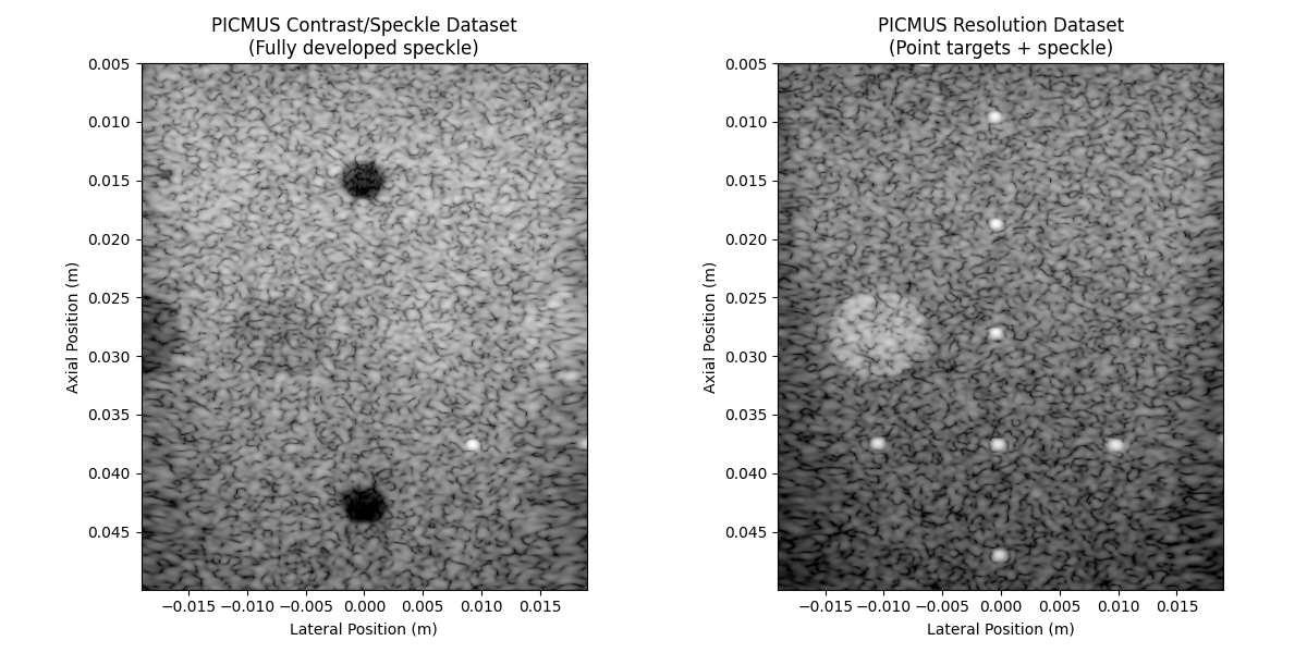
Load PICMUS datasets [3] for comparison

# Load contrast/speckle dataset (contains fully developed speckle regions)
image_contrast, scan_contrast = load_uff_dataset("picmus_contrast_experiment")
image_contrast = image_contrast.T

# Load resolution dataset (contains point targets and speckle)
image_resolution, scan_resolution = load_uff_dataset("picmus_resolution_experiment")
image_resolution = image_resolution.T

Visualize datasets side by side

fig, axes = plt.subplots(1, 2, figsize=(12, 6))

# Contrast/speckle dataset
extent_contrast = [
    scan_contrast.x_axis.min(),
    scan_contrast.x_axis.max(),
    scan_contrast.z_axis.max(),
    scan_contrast.z_axis.min(),
]
axes[0].imshow(db_zero(image_contrast), cmap="gray", extent=extent_contrast, vmin=-60, vmax=0)
axes[0].set_title("PICMUS Contrast/Speckle Dataset\n(Fully developed speckle)")
axes[0].set_xlabel("Lateral Position (m)")
axes[0].set_ylabel("Axial Position (m)")

# Resolution dataset
extent_resolution = [
    scan_resolution.x_axis.min(),
    scan_resolution.x_axis.max(),
    scan_resolution.z_axis.max(),
    scan_resolution.z_axis.min(),
]
axes[1].imshow(db_zero(image_resolution), cmap="gray", extent=extent_resolution, vmin=-60, vmax=0)
axes[1].set_title("PICMUS Resolution Dataset\n(Point targets + speckle)")
axes[1].set_xlabel("Lateral Position (m)")
axes[1].set_ylabel("Axial Position (m)")

plt.tight_layout()

Define ROI locations for speckle analysis

# Following Perdios et al., we use regions of approximately 10λx10λ
# Assuming center frequency ~5 MHz and speed of sound ~1540 m/s
# λ ≈ 1540/5e6 ≈ 0.3 mm, so 10λ ≈ 3 mm radius
roi_radius = 0.003  # 3 mm radius

# Equation S9 from Perdios et al. [2]_ and Equation 4 from Burckhardt [1]_
theoretical_rayleigh_snr = np.sqrt(np.pi / (4 - np.pi))

# Define ROI locations for different types of regions
roi_specs = [
    {
        "name": "Fully Developed Speckle (contrast dataset)",
        "dataset": "contrast",
        "center": (-0.005, 0.035),
        "expected_snr": theoretical_rayleigh_snr,
        "description": "Homogeneous speckle region",
    },
    {
        "name": "Fully Developed Speckle (resolution dataset)",
        "dataset": "resolution",
        "center": (0.008, 0.030),
        "expected_snr": theoretical_rayleigh_snr,
        "description": "Homogeneous speckle region",
    },
    {
        "name": "Point Target Region",
        "dataset": "resolution",
        "center": (0.000, 0.0275),  # Near a point target
        "expected_snr": None,  # Should deviate from Rayleigh
        "description": "Point target + speckle",
    },
    {
        "name": "Lesion Boundary",
        "dataset": "contrast",
        "center": (-0.0025, 0.028),  # Near lesion boundary
        "expected_snr": None,  # Mixed statistics
        "description": "Lesion boundary region",
    },
]

Compute SNR for each ROI

results_data = []

for spec in roi_specs:
    # Select the appropriate dataset and scan
    if spec["dataset"] == "contrast":
        image = image_contrast
        scan = scan_contrast
        extent = extent_contrast
    else:
        image = image_resolution
        scan = scan_resolution
        extent = extent_resolution

    # Create ROI mask
    mask = build_mask(
        position=spec["center"],
        dimension=roi_radius,
        x_axis=scan.x_axis,
        z_axis=scan.z_axis,
        shape="circle",
    )

    # Extract values in ROI
    roi_values = image[mask]

    # Compute SNR (function handles complex data internally)
    snr_linear = snr(roi_values, db=False)
    snr_db = snr(roi_values, db=True)

    # Calculate deviation from theoretical Rayleigh SNR if expected
    if spec["expected_snr"] is not None:
        deviation = abs(snr_linear - spec["expected_snr"])
        deviation_percent = (deviation / spec["expected_snr"]) * 100
    else:
        deviation = None
        deviation_percent = None

    results_data.append({
        "ROI": spec["name"],
        "Dataset": spec["dataset"],
        "SNR (linear)": snr_linear,
        "SNR (dB)": snr_db,
        "Expected SNR": spec["expected_snr"],
        "Deviation": deviation,
        "Deviation (%)": deviation_percent,
        "Description": spec["description"],
        "mask": mask,
        "center": spec["center"],
        "extent": extent,
        "image": image,
    })

Display results table

results_df = pd.DataFrame(results_data)

print("=== SNR Analysis Results ===")
display_cols = ["ROI", "Dataset", "SNR (linear)", "SNR (dB)", "Expected SNR", "Deviation (%)"]
print(results_df[display_cols].round(3))

print(f"\nTheoretical Rayleigh SNR: {theoretical_rayleigh_snr:.3f}")

for _, row in results_df.iterrows():
    if row["Expected SNR"] is not None:
        if row["Deviation (%)"] < 10:
            status = "✅ Good agreement with theory (Rayleigh distribution)"
        elif row["Deviation (%)"] < 20:
            status = "⚠️  Moderate deviation from theory"
        else:
            status = "❌ Significant deviation from theory"
        print(f"{row['ROI']}: SNR = {row['SNR (linear)']:.3f}, {status}")
    else:
        print(f"{row['ROI']}: SNR = {row['SNR (linear)']:.3f} (non-Rayleigh distribution)")

=== SNR Analysis Results ===
                                            ROI  ... Deviation (%)
0    Fully Developed Speckle (contrast dataset)  ...         2.189
1  Fully Developed Speckle (resolution dataset)  ...         1.115
2                           Point Target Region  ...           NaN
3                               Lesion Boundary  ...           NaN

[4 rows x 6 columns]

Theoretical Rayleigh SNR: 1.913
Fully Developed Speckle (contrast dataset): SNR = 1.955, ✅ Good agreement with theory (Rayleigh distribution)
Fully Developed Speckle (resolution dataset): SNR = 1.892, ✅ Good agreement with theory (Rayleigh distribution)
Point Target Region: SNR = 0.534, ❌ Significant deviation from theory
Lesion Boundary: SNR = 1.520, ❌ Significant deviation from theory

Visualize ROIs and SNR measurements

fig, axes = plt.subplots(2, 2, figsize=(15, 12))
axes = axes.flatten()

for i, (_, row) in enumerate(results_df.iterrows()):
    ax = axes[i]

    # Display the image
    ax.imshow(db_zero(row["image"]), cmap="gray", extent=row["extent"], vmin=-60, vmax=0)

    # Overlay ROI circle
    circle = Circle(row["center"], roi_radius, fill=False, color="red", linewidth=2, linestyle="--")
    ax.add_patch(circle)

    # Add SNR annotation
    ax.text(
        row["center"][0],
        row["center"][1] - 0.008,
        f"SNR = {row['SNR (linear)']:.2f}",
        ha="center",
        va="top",
        color="white",
        fontweight="bold",
        bbox={"boxstyle": "round,pad=0.3", "facecolor": "black", "alpha": 0.8},
    )

    ax.set_title(f"{row['ROI']}\n{row['Description']}")
    ax.set_xlabel("Lateral Position (m)")
    ax.set_ylabel("Axial Position (m)")

plt.tight_layout()

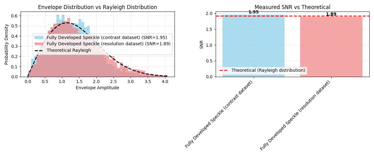
Statistical analysis of speckle regions

# Focus on the fully developed speckle regions
speckle_rows = results_df[results_df["Expected SNR"].notna()]

fig, axes = plt.subplots(1, 2, figsize=(12, 5))

colors = ["skyblue", "lightcoral"]
for i, (_, row) in enumerate(speckle_rows.iterrows()):
    # Extract ROI values and convert to envelope (magnitude)
    roi_values_complex = row["image"][row["mask"]]
    roi_values = np.abs(roi_values_complex)  # Take envelope for histogram

    # Create histogram of envelope values
    axes[0].hist(
        roi_values,
        bins=50,
        alpha=0.7,
        density=True,
        color=colors[i],
        label=f"{row['ROI']} (SNR={row['SNR (linear)']:.2f})",
    )

# Overlay theoretical Rayleigh distribution
x_theory = np.linspace(0, roi_values.max(), 1000)
# For comparison, use sigma that gives the same mean as our data
sigma_rayleigh = np.mean(roi_values) / np.sqrt(np.pi / 2)
rayleigh_pdf = (x_theory / sigma_rayleigh**2) * np.exp(-(x_theory**2) / (2 * sigma_rayleigh**2))
axes[0].plot(x_theory, rayleigh_pdf, "k--", linewidth=2, label="Theoretical Rayleigh")

axes[0].set_xlabel("Envelope Amplitude")
axes[0].set_ylabel("Probability Density")
axes[0].set_title("Envelope Distribution vs Rayleigh Distribution")
axes[0].legend()
axes[0].grid(True, alpha=0.3)

# SNR comparison bar chart
roi_names = [row["ROI"] for _, row in speckle_rows.iterrows()]
snr_values = [row["SNR (linear)"] for _, row in speckle_rows.iterrows()]

bars = axes[1].bar(roi_names, snr_values, alpha=0.7, color=colors)
axes[1].axhline(
    y=theoretical_rayleigh_snr,
    color="red",
    linestyle="--",
    linewidth=2,
    label="Theoretical (Rayleigh distribution)",
)
axes[1].set_ylabel("SNR")
axes[1].set_title("Measured SNR vs Theoretical")
axes[1].legend()
axes[1].grid(True, alpha=0.3)

# Add value labels on bars
for bar, value in zip(bars, snr_values):
    height = bar.get_height()
    axes[1].text(
        bar.get_x() + bar.get_width() / 2.0,
        height + 0.01,
        f"{value:.2f}",
        ha="center",
        va="bottom",
        fontweight="bold",
    )

plt.xticks(rotation=45, ha="right")
plt.tight_layout()

%% Show all figures (if run as a script)

plt.show()

Best Practices for SNR Measurement

Based on the analysis above, here are key guidelines for SNR measurement:

1. ROI Size Guidelines:

   • Use regions of approximately 10λx10λ for adequate statistical sampling

   • For 5 MHz transducers: ≈3mm x 3mm ROI provides good sampling

   • Larger ROIs provide more stable statistics but may include spatial variations

2. Region Selection Criteria:

   • Choose homogeneous speckle areas away from boundaries

   • Avoid edges with incomplete plane wave coverage

3. Regions to Avoid:

   • Lesion edges (mixed Rayleigh/non-Rayleigh statistics)

   • Point targets (coherent scattering, non-Rayleigh)

   • Field edges (incomplete acoustic data)

   • Areas with obvious artifacts

4. Expected Values for Quality Assessment:

   • Fully developed speckle: SNR ≈ 1.91 (Rayleigh distribution) [1] [2]

   • Point targets: SNR significantly < 1.91

   • Mixed regions: Variable SNR depending on content mixture

5. Clinical and Research Applications:

   • Speckle quality assessment in different tissue types

   • Beamforming algorithm evaluation and optimization

   • System validation and quality control